05. Faceting in Two Directions

Faceting for Multivariate Data

In the previous lesson, you saw how FacetGrid could be used to subset your dataset across levels of a categorical variable, and then create one plot for each subset. Where the faceted plots demonstrated were univariate before, you can actually use any plot type, allowing you to facet bivariate plots to create a multivariate visualization.

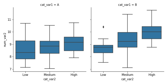
g = sb.FacetGrid(data = df, col = 'cat_var1', size = 4)
g.map(sb.boxplot, 'cat_var2', 'num_var2')

The faceted box plot suggests a slight interaction between the two categorical variables, where, in level B of "cat_var1", the level of "cat_var2" seems to be have a larger effect on the value of "num_var2", compared to the trend within "cat_var1" level A.

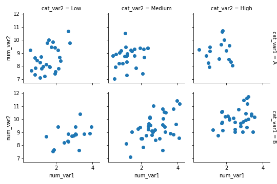
FacetGrid also allows for faceting a variable not just by columns, but also by rows. We can set one categorical variable on each of the two facet axes for one additional method of depicting multivariate trends.

g = sb.FacetGrid(data = df, col = 'cat_var2', row = 'cat_var1', size = 2.5,
                margin_titles = True)
g.map(plt.scatter, 'num_var1', 'num_var2')

Setting margin_titles = True means that instead of each facet being labeled with the combination of row and column variable, labels are placed separately on the top and right margins of the facet grid. This is a boon, since the default plot titles are usually too long.